Convert Horizontal Data to Vertical Data 1

[Topcat04]

Hi There
I'm looking for help to convert horizontal data entered in a workbook for recording sales to vertical data please. I'm hoping someone with VBA expertise will be able to help.
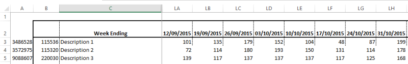
In row 2 are the weekly dates recorded in Column D to Column LH
In row 3 to 130 are products with their sales recorded by week (column D to LH)
Column A has a product identifier Code
Column B has an internal product identifier code
Column C has a product description.

Week Ending 10/10/2009 17/10/2009 24/10/2009 31/10/2009 07/11/2009
218118 330046 Description 1 316 617 555 580 819
204866 330015 Description 2 231 194 253 391 322
218117 330048 Description 3 200 361 321 323 412

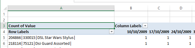
I'm hoping to be able to get the data in a vertical format so that
Column A, B, C remains the Same,
Column D has the weekly sales
Colum E has the weekly Date

Look forward to your help,
Thanks
- TC

 

[SkipVought]

Hi,

Unless this is a repeatable task, not VBA required. Otherwise, perform this manually while recording:

1) SELECT the data you want to transpose. It can be more than one column if applicable.

2) COPY

3) Select the target location

4) Right-Click and select PASTE SPECIAL--TRANSPOSE.

Post back with your recorded code if you need help customizing.

Skip,
[sub]
Just traded in my OLD subtlety...
for a NUance![/sub]

 

[Topcat04]

Hi Skip
Thanks for the response,
I expected it to be a VBA as it is 317 columns of data.
For each column of data the product identifier, description, weekly sales needs to be copied under each other and the date pasted for each entry that week.
With 127 products by 317 columns, that's quite a lot of manual pasting which is why I was hoping some code would do the job instead.
Hope that makes some more sense,
thanks for your reply,
- TC

 

[SkipVought]

Well then you have not adequately described your data structure!

Can you upload a representative sample? Your description makes no sense to me.

And where is this apparently horrible data coming from? Surely there's a better source?

Skip,
[sub]
Just traded in my OLD subtlety...
for a NUance![/sub]

 

[Topcat04]

Hi Skip
the data is inherited and I am looking to make a table of it so that it will be in a better structure. I cant change the source as its a one off inherited.

As described the dates go from Column D to Column LH
the products go from row 3 to 130

I'm looking to get it so that it looks more like this... (just used three test codes and descriptions but this would repeat for the 127 products for each weekly date)

Hope that makes more sense?
appreciate your help!
- TC

 

[SkipVought]

Okay, so you want to NORMALIZE your data, which involves transposing.

So my thought is to use this technique faq68-5287.

This sounds like an ANNUAL task. You may be able to automate it, but the process should only take a few minutes, maybe 15 at the most.

The only caveat is that first you ought to do these things in order that the ROW DATA (that is your GMSKU, PASKU & Description data) is ALL concatenated into ONE COLUMN, from row 1 to row 128. Oh yes, I deleted the first row! Why do people put empty rows at the top of a table??? I'd use the | delimiter. Makes it simple to break them back to 3 columns using Data > Text to Columns -- DELIMITED, after the normalization process. So in your table, insert a column after C for the concatenated data. Then reference C1 to LI128 or whatever row in the normalization steps.

So after you get the row data into one column, perform the normalization process, then shift the column & value columns 2 to the right to make room for Text to Columns. Finally, fix your headings.

Skip,
[sub]
Just traded in my OLD subtlety...
for a NUance![/sub]

 

[SkipVought]

BTW, this is what the raw normalization result looks like.
[pre]
Row Column. Value
218118|330046|Description 1 10/10/2009 316
218118|330046|Description 1 17/10/2009 617
218118|330046|Description 1 24/10/2009 555
218118|330046|Description 1 31/10/2009 580
218118|330046|Description 1 07/11/2009 819
204866|330015|Description 2 10/10/2009 231
204866|330015|Description 2 17/10/2009 194
204866|330015|Description 2 24/10/2009 253
204866|330015|Description 2 31/10/2009 391
204866|330015|Description 2 07/11/2009 322
218117|330048|Description 3 10/10/2009 200
218117|330048|Description 3 17/10/2009 361
218117|330048|Description 3 24/10/2009 321
218117|330048|Description 3 31/10/2009 323
218117|330048|Description 3 07/11/2009 412
[/pre]


Skip,
[sub]
Just traded in my OLD subtlety...
for a NUance![/sub]

 

[Topcat04]

Hi Skip
I was hopeful this was going to work and in theory it should do, however trying to normalize the data, it breaks down at step 6, as values is set to Count of Value and the data is the same as it was on the previous work sheet, other than it has blue shading on row 3 and 4 and a dropdown filter on Row labels in A4 and Column Labels in B3.

In the PivotTable Fields sidebar, if I drag column from Columns and Row from Rows, all I get is the following

Not sure which part I misunderstood. I'm using Excel 2016.
Thanks for your continued support,
- TC

 

[SkipVought]

Your last pic is EXACTLY what you ought to see in the Pivot Table.

The NEXT step is to double-click in A4.

You're almost there!

Skip,
[sub]
Just traded in my OLD subtlety...
for a NUance![/sub]

 

[Topcat04]

Awesome!!
Thank you for your patience and help, we have the desired result!!
really appreciate it,
- TC

 

[SkipVought]

Great. Keep this one in your hip pocket

Skip,
[sub]
Just traded in my OLD subtlety...
for a NUance![/sub]