Top 50 Items (Sales) PivotChart with Slicer that Groups 10 at a Time

[ryplew]

Hello!

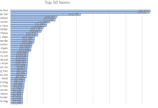
I have a Clustered Bar PivotChart showing the top 50 sales items. Of course, 50 items at once is far too many to show on a chart. Yet, I am tasked with showing the top 50 sales items graphically. My thought would be to have a slicer to where I could select 1 - 10, 11 - 20, 21 - 30, 31 - 40, and 41 - 50. However I am not coming up with any ideas of how to do this. When I use a slicer based off of sales, I am on able to use a dollar amount. I'd like to base the slicer off of a selection of the top 50. Perhaps I may need to go the VBA route?

PivotTable Info:
Has two columns: Item and Sales
Is filtered for the Top 50 and sorted highest to lowest

 

[SkipVought]

Hi,

What is there to cluster? You have only ITEM on the Category axis and SALES on the Value axis. There's nothing to cluster as far as you have indicated!

I'd use a COLUMN chart.

I assume that your PivotTable source data has multiple rows per Item. If it 1:1, then there's no need for a PivotTable/PivotChart. Just plot the source data directly..

I'd use controls to change the number of Items displayed on the chart, and a slider to change the starting Item.

 

[ryplew]

Hi Skip!

My apologies on referring to a "Clustered" Bar Chart. You are correct in that I am not even utilizing the "Clustered" feature of the chart. It is simply a Bar Chart.

I would still like to use a Bar Chart if possible as I like how the data is represented with a vertical hierarchy as opposed to a horizontal one.

Yes, my source data has multiple rows per Item. And, there are additions made to the source data monthly.

With my PivotTable filtered to display Top 50 Items, my Pivot Chart looks something like the image below. Not all 50 Items are shown and it is very hard to read. My initial thought is to use a selector to display groups of 10 at a time so that it looks cleaner.

I am afraid that I am not sure how to use a control to change the number of Items displayed on the chart, nor how to use a slider to change the starting item (being the 1st, 11th, 21st, 31st, or 41st Item of the Top 50).

 

[combo]

You have exactly 50 items displayed, not all names are displayed in y-axis labels. You can change font and/or chart orientation (with vertical text) to have more room for names.

combo

 

[SkipVought]

I'd try using the OFFSET() function as the range for the chart.

Arguments:
1) fixed at the upper LH cell in PT data
2) this will be a reference to a cell that you will enter the offset row ( minus 1) for the beginning value for your chart to display
3) 0
4) this will be a reference to a cell tjat you will enter the number of data points you want to display
5) 1

You can just enter values into these 2 cells or use a control to enter the values.

 

[ryplew]

Thanks for the reply, combo!

I am aware that all of the labels are not showing and that they can be formatted to all fit. However, I would like to not have to show ALL 50 at one time, because every thing becomes quite condensed and hard to read. I would like to make this one chart on a dashboard. So showing 10 at a time would be ideal with the user having the option to select the next set of 10 and so on.

 

[ryplew]

That sounds interesting, Skip. I will certainly give that a go. Thank you!

 

[SkipVought]

Did you see my previous post?

 

[zelgar]

I'm not too familiar with Pivot tables, but couldn't you just have another sheet do a calculation to sum up the values for the data for each of the 10 items for items 1-10, 11-20, 21-30 ... and graph the results? Alternately, using the RANK & SUMIF functions you could perform this on an unsorted spreadsheet.

 

[SkipVought]

The OP wants to DISPLAY 1-10 etc

 

[zelgar]

I think he easiest option would be to have a different sheet to get the data he wants from the Pivot Table.
1. In the Pivot Table, use the RANK function to determine the rank of each item (e.g., in col H =RANK(G2, G$2:G$500, 1))
2. Have a cell (e.g. B1) that used Data Validation for the Starting Value (e.g., 1, 11, 21, etc.)
2. Have the next 10 cells getting data from the original sheet (e.g., let's say the data is in Sheet1 cells H2:H100)
Cell A2 = "Item", Cell B2="Value"
Cell A3 = INDEX(A$2:A$500,MATCH(B1,H$2:H$500,1),1)
Cell A4 = INDEX(A$2:A$500,MATCH(B1+1,H$2:H$500,1),1)
.
.
Cell A12 = INDEX(A$2:A$500,MATCH(B1+9,H$2:H$500,1),1)

Cell B3 = INDEX(G$2:G$500,MATCH(B1,H$2:H$500,1),1)
Cell B4 = INDEX(G$2:G$500,MATCH(B1+1,H$2:H$500,1),1)
.
.
.
Cell B12 = INDEX(G$2:G$500,MATCH(B1+9,H$2:H$500,1),1)

3. Make a graph based upon the above items

 

[SkipVought]

Okay, I forgot that the Chart SourceData for a PivotChart is not editable.

So here's an approach:
[tt]
ADD a "Top 10 Filter on your PivotTable
Turn on your Macro Recorder and record CHANGING the "Top 10" filter to another value
Post your recorded code here to get help modifying your code (alt+F11 toggles between the the VB Editor and the sheet)
[/tt]

We can use a cell on your sheet to enter the number of rows to display.

 

[ryplew]

Thanks, Skip. Here is the code you asked for...

Sub ChangeTop10to50()

    ActiveSheet.PivotTables("PivotTable1").PivotFields("Item / Item Description"). _
        ClearAllFilters
    ActiveSheet.PivotTables("PivotTable1").PivotFields("Item / Item Description"). _
        PivotFilters.Add2 Type:=xlTopCount, DataField:=ActiveSheet.PivotTables( _
        "PivotTable1").PivotFields("Sum of Sales $"), Value1:=50
End Sub

 

[SkipVought]

Okay. In my sheet, the cell immediately above the cell containing "Column Labels" is [highlight #FCE94F]H1[/highlight]. You put [highlight #FCE94F]your cell reference[/highlight] in there. BTW, this macro is not to change the top 10 to 50. Its to display ANY NUMBER of points you decide to enter.

Sub ChangeTop10()

    ActiveSheet.PivotTables("PivotTable1").PivotFields("Item / Item Description"). _
        ClearAllFilters
    ActiveSheet.PivotTables("PivotTable1").PivotFields("Item / Item Description"). _
        PivotFilters.Add2 Type:=xlTopCount, DataField:=ActiveSheet.PivotTables( _
        "PivotTable1").PivotFields("Sum of Sales $"), Value1:=ActiveSheet.Range("[highlight #FCE94F]H1[/highlight]").Value
End Sub

But there's one more thing to. Right-click the Sheet TAB and select View Code. This is the VBA Code Editor. You can toggle between the editor and the sheet using alt+F11.

Above the code window to the left you'll see (General) in a Drop Down. Click the DD & select Worksheet.

Above the code window to the right you'll see a number so Sheet Events in a Drop Down. Click the DD & select Change.

Add THIS code. Remember to put your cell reference [highlight #FCE94F]here[/highlight].

Private Sub Worksheet_Change(ByVal Target As Range)
[b]    If IsNumeric([H1]) Then
        If Not Intersect(Target, [[highlight #FCE94F]H1[/highlight]]) Is Nothing Then
            PlotRows
        End If
    End If
[/b]End Sub

And on your sheet, [highlight #FCE94F]HERE[/highlight] is where you can ENTER 10 or 15 or 50 or however many points you want to display.