Excel Vlookup

[Cpreston]

Hi

I have a sheet with information about costs

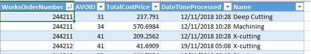
I also have another sheet with some information and I want to populate the costs into this sheet. They have works order number as the key yo match with.

In sheet 1 the works order number may have 3 different costs , or more or less, depending on what processes it goes through. Example is in the screen shot below.

I have used this vlookup to get the data =IFERROR(VLOOKUP(A:A,'Paint Data'!A:E,3,FALSE),"")

This only brings back the first result of 237.791, how can I get it so it shows the other 2, if that is at all possible, Thanks in advance.

 

[combo]

I don't know the data structure you have, but for me VLOOKUP is not a good tool for this.
In excel 2019/365 you may consider FILTER function.
In excel 2016+ Power Query may be used to join tables, input parameters and output to table or pivot table (requires refreshing after changing input).

combo

 

[Cpreston]

You may be right, one thing that would work is if I could sum the vlookup, any ideas how I change the formulae to do this? I have googled a bit but cant find something suitable.
n
=IFERROR(VLOOKUP(A:A,'Paint Data'!A:E,3,FALSE),"")

Thanks

 

[combo]

For single sum use SUMIF, for multiple criteria SUMIFS.

combo

 

[Cpreston]

Tried both but my syntax just is not accepted

=SUMIF(VLOOKUP([WorksOrderNumber],'Paint Data'!A:C,3,FALSE),"") , I have tried to change it round but no luck

=SUMIFS(VLOOKUP([WorksOrderNumber],'Paint Data'!A:C,3,FALSE),"") it says I have entered to few arguments of it.

Any ideas on the syntax please

 

[Cpreston]

Go this far

=SUMIFS(Table3[[#Headers],[WorksOrderNumber]],VLOOKUP('Paint Data'!A:A,3,FALSE),'Paint Data'!C:C)

But still not working, any ideas anyone.

 

[Cpreston]

used this in the end =SUMIF('Paint Data'!A:A,[@WorksOrderNumber],'Paint Data'!C:C)

However, this just gives me the Total Process Cost , I need to show them individually, I will look into your power quesry method. Thanks

 

[strongm]

VLOOKUP cannot return multiple values.

But this looks to me like it could be solved with a pivot table

 

[SkipVought]

@cpreston, forget about VLOOKUP!!! You seem to be fixated on that function.

From what you have indicated a simple SUMIF is all you need, if indeed all that is required is one WorkOrderNumber to sum the TotalCostPrice.

Personally, I'd rather use SUMPRODUCT in place of SUMIF or SUMIFS or COUNTIF or COUNTIFS. But that's just me.

Skip,
[sub]
Just traded in my OLD subtlety...
for a NUance![/sub]
"The most incomprehensible thing about the universe is that it is comprehensible" A. Einstein

 

[SkipVought]

However, this just gives me the Total Process Cost , I need to show them individually,

That sounds like a simple PivotTable.

Skip,
[sub]
Just traded in my OLD subtlety...
for a NUance![/sub]
"The most incomprehensible thing about the universe is that it is comprehensible" A. Einstein

 

[mintjulep]

Agree with pivot table.

The new XLOOKUP() might be able to return multiple results. I haven't fully come to grips with its use yet.

 

[combo]

A tip with new dynamic arrays, if you have 365:

https://theexcelclub.com/excel-dynamic-arrays-a-new-way-to-model-your-excel-spreadsheets/

combo

 

[SkipVought]

???

I also have another sheet with some information and I want to populate the costs into this sheet. They have works order number as the key yo match with.

Well if you have "another sheet" that already has "works order number as the key yo match with" then the SUMIF formula will do the job.

???
You are giving mixed signals.

Skip,
[sub]
Just traded in my OLD subtlety...
for a NUance![/sub]
"The most incomprehensible thing about the universe is that it is comprehensible" A. Einstein