Tek-Tips is the largest IT community on the Internet today!

Members share and learn making Tek-Tips Forums the best source of peer-reviewed technical information on the Internet!

  • Congratulations IamaSherpa on being selected by the Tek-Tips community for having the most helpful posts in the forums last week. Way to Go!

Excel: Return the neighbouring cell ref using a formula 2

Status
Not open for further replies.

DAmoss

Technical User
Jul 23, 2003
169
GB
Hi,

I have written the following little formula which works well except for a known problem which I've now discovered whilst trawling the net:

=OFFSET(INDIRECT(CELL("address")),0,1)

The above formula always checks the last cell that was processed and not the one I always want it to check, in this case the cell I always want is the one directly to the right of whichever cell I assign this formula to.

I don't want to put actual cell references in the formula as I'm using it as part of some 'Conditional Formatting' that I've set up. I am highlighting two neighbouring figures if they are not the same value.

Can anyone give me some pointers as to how to target the required cell without typing in its direct reference. The formula has to work out its current cell ref and then look at the value in the one directly to right of it.

Thanks in advance.
 
Please explain what you are trying to achieve with your entire formula?

Cheers, Glenn.

Beauty is in the eye of the beerholder.
 
Don't worry about references in conditional formatting, if they are not absolute, keep relative referencing (like in copying formulas).

combo
 
I agree with combo ... by the sound of it simple relative referencing should work.

Cheers, Glenn.

Beauty is in the eye of the beerholder.
 
Quick Explanation:

The formula returns the value contained in the cell directly to the right of cell that has the Conditional Formatting formula. In my Conditional Formatting condition I am using the following choice:

Cell value is not equal to =OFFSET(INDIRECT(CELL("address")),0,1)

This highlights the cell doing the checking in lightblue if it is not equal to the cell next to it ... except it works first time but then doesn't work as it should due to the CELL() function referring to the last value accessed rather than the one I want.

Try it and you will see what I mean, all my cells with the conditional formatting light up (even when they have the same value next to them)

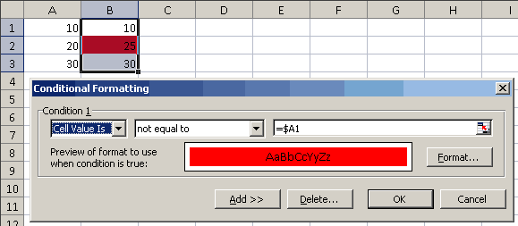
10 10
20 25 << Highlight value 20
30 30

 
And why aren't you doing a simple reference to the cell in column B like, select A2:B4, Condition of:
Cell Value is not equal to $B2

Cheers, Glenn.

Beauty is in the eye of the beerholder.
 
I'm not doing a simple reference because I have thousands of values that I would have to reference individually in the 'Conditional Formatting' option. When you set one up and copy it down, it still references the original cell in all cases. I would have to go into each one and manually alter them ... hence I need a formula to this instead.

Can anyone give me some help with this problem, is there a way to do what I'm asking or should I just go back to manually highlighting the two cells that don't match?
 
Remove unnecessary '$' sign(s) in CF references. Next, if you copy such cell with CF, references in CF formulas of copied cells will change according to general copying rules. It is possible to extend conditional formatting to selected region.
Follow Glenn's advice and test it with simple rules in a small range.

combo
 
Solved: Not a problem now as I've solved it by using any of the following formulas depending on which neighbouring value I want to look at:

NextCellUp:
= INDIRECT("R[-1]C", 0)

NextCellDown:
= INDIRECT("R[1]C", 0)

NextCellLeft:
= INDIRECT("RC[-1]", 0)

NextCellRight:
= INDIRECT("RC[1]", 0)

eg. Cell value is not equal to = INDIRECT("RC[1]", 0)

Ussing the 'NextCellRight' formula does the trick and it also allows me to copy it down accordingly, it works beautifully in the 'Conditional Formatting' option as shown above.
 
When you set one up and copy it down, it still references the original cell in all cases.

NO, that is not the case. Use relative references, as combo and I suggest and all would be fine, without the need for complex solutions.

Cheers, Glenn.

Beauty is in the eye of the beerholder.
 
Hang on ... I come up with a solution that actually works and you say 'NO, that is not the case' ... It WORKS, Am I missing something here? My original question stated that I did not want any cell references to be used in my formula.

A working solution is good thing in my eyes (be it slightly complex or not), if you are saying there is a far better and simpler way to do this then please give a working example and not just a running commentary on my working 'wrong' way.

I am a great believer in actually showing people how to do things and not just trying to point them in the right direction.
 
ok.
conditionalrelative.gif
 
original post said:
The above formula always checks the last cell that was processed and not the one I always want it to check, in this case the cell I always want is the one directly to the right of whichever cell I assign this formula to.

Whilst totally agreeing with the simpler solutions suggested by others, I note that looking at excel help would also have provided a solution:- just use the second, optional parameter of Cell:.
excel help said:
Syntax CELL(info_type,reference)
Reference is the cell that you want information about. If omitted, information specified in info_type is returned for the last cell that was changed.


Gavin
 
Just to end this one once and for all:

Combo & Gruuuu
I now know what you have stated is correct, easier and works, thank you for the example as well. Now I can actually see how it's done!

Cheers
 
Status
Not open for further replies.

Part and Inventory Search

Sponsor

Back
Top