Excel Pivot Table - Combine Values into a single row

[remeng]

Hi,

I have a pivot table with two value columns. The data changes each day. One of the columns tells the user the total number (count of Required Quantity) of hardware packs that are required. The second column sums the total parts within the hardware packs (Sum of Comp_Qty). I am trying to create a single line of the hardware pack number and leave the component level as is.

The data is currently correct for both the quantity of hardware packs to make and the total number of components in all the hardware packs. This information is used by our warehouse to pick the total components and create the total count of the hardware packs.

Here is the current configuration that is incorrect.





I need it to show SHIP HDW UNTZ FLATBR KIT = 24 and the Sum of Comp_Qty to stay the same.


Here is an example of what I need.



When I try and move the Required Quantity field to the left of Component, it changes the value from 24 (correct) to 1 (incorrect).





Does anyone know how I can make my Pivot Table show the values in the format I need?

Thank you for the help!

Mike

 

[mintjulep]

So each 12012-1133-00 kit contains:
2 x 18907-6791-34
1 x 19898-0153-00
16 x 19917-4387-36

???

In the underlying data, where are those 2, 1 and 16 factors?

In the underlying data, where is there a 24 indicating that you need 24 kits?

 

[mintjulep]

Like this:
Data in left 4 columns, Pivot table in the right 5 columns.

Kit	Kits used per day	Part	parts per kit			Kit	Kits used per day	Part	Sum of parts per kit	Sum of Parts used per day
K1	24​	P1	2​			K1
K1	24​	P2	1​				24​
K1	24​	P3	16​					P1	2​	48​
								P2	1​	24​
								P3	16​	384​

Where:

Sum of Parts used per day

='Kits used per day' *'parts per kit'

 

[mintjulep]

Potentially more useful to calculate 'parts per day per kit' in the data.

Kit	Kits used per day	Part	parts per kit	Parts per day per kit
K1	24​	P1	2​	48​
K1	24​	P2	1​	24​
K1	24​	P3	16​	384​
K2	5​	P1	3​	15​
K2	5​	P2	4​	20​
K2	5​	P4	1​	5​

Then you can use a pivot to report kit-wise:

Kit	Kits used per day	Part	Parts Used per Day per Kit
K1
	24​
		P1	48​
		P2	24​
		P3	384​
K2
	5​
		P1	15​
		P2	20​
		P4	5​

And a pivot to report part-wise:

	Total Parts per day
P1	63​
P2	44​
P3	384​
P4	5​

 

[SkipVought]

Hi,

I have a pivot table with two value columns. The data changes each day. One of the columns tells the user the total number (count of Required Quantity) of hardware packs that are required. The second column sums the total parts within the hardware packs (Sum of Comp_Qty). I am trying to create a single line of the hardware pack number and leave the component level as is.

The data is currently correct for both the quantity of hardware packs to make and the total number of components in all the hardware packs. This information is used by our warehouse to pick the total components and create the total count of the hardware packs.

Here is the current configuration that is incorrect.

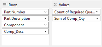
View attachment 649

View attachment 650

I need it to show SHIP HDW UNTZ FLATBR KIT = 24 and the Sum of Comp_Qty to stay the same.


Here is an example of what I need.

View attachment 651

When I try and move the Required Quantity field to the left of Component, it changes the value from 24 (correct) to 1 (incorrect).

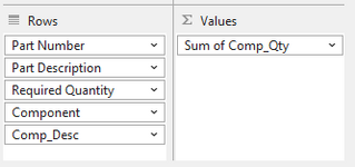
View attachment 652

View attachment 653

Does anyone know how I can make my Pivot Table show the values in the format I need?

Thank you for the help!

Mike

As mintjulep has stated, it ALL depends on "the underlying data"

Data is $money.

Show me the $money!

 

[remeng]

Hi,

Thanks for the quick replies. So the data is coming from two different data sources. Both are combined using Power Query.

I've tried using combine Pivots prior without any luck, hence utilizing Power Query. Also, the data source info is dynamic, so I am pulling the raw data from other files.

Here's a screenshot of the raw data. The Required Quantity of Packs = 24 and the sum total of Comp_Qty = 384 for the screws.

Each Pack has 16 screws.



There are other Components in the hardware pack, but the premise is still the same.

 

[mintjulep]

So what's wrong in your first pivot?


You get the correct Component Quantities.
You get the number of kits.
As a bonus you get confirmation that each component has been used in the same number of kits.

 

[mintjulep]

The Required Quantity of Packs = 24

I think your problem is that the data doesn't contain this requirement.

You have 24 rows, indicating that 16 screws have been used 24 times.

There's nothing that says 24 is the correct number.

 

[mintjulep]

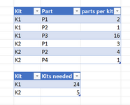
Start with two tables. One to define what parts are in each kit, a second to define how many of each kit are required.


Then use Power Query LeftOuter join to get this table:


Then pivot that to get what you want:

 

[remeng]

Hi Mintjulep,

I created the tables as you suggested, but I think my Power Query merge LeftOuter Join isn't correct. The numbers just don't match the data correctly.

Here is my raw data. What am I doing wrong?

Thanks for the help!

 

[mintjulep]

Hi remeng,

Thanks for attaching the spreadsheet.

However, the spreadsheet that you attached is quite different from everything that you've posted so far:

1. It introduces "Serial Number" that hasn't been discussed at all.
2. In the Component table, the listed "Comp_Qty" is 1 for every serial number.
3. In the Hardware Packs table, the listed "Required Quantity" is 1 for every row.

So, it's not at all clear to me what you are trying to do.

Please step us through the process.

1. In the beginning we have:
   1. A
   2. B
   3. C
2. A user needs to use A, B and C to do:
   1. X
   2. Y
   3. Z
3. At the end we have....

 

[remeng]

Hi MJ,

1) The SN is just used like an index key to cross reference the kits and make sure the count / sum values are correct between the number of kits and the number of parts inside the kits.
2) The kits are made of the following

Part Number

• 12016-1023-00 (SHIP HDW GLIDES 6)
  • 19962-0002-00 (HDW PKG GLIDES(6) = QTY 1
  • 19898-0153-00 BAG PLS ORANGE 24X10 = QTY 1

For each kit (Part Number) there is one set of glides (component) and one bag (component)



Hope that helps

 

[mintjulep]

Please step us through the process.

1. In the beginning we have:
   1. A
   2. B
   3. C
2. A user needs to use A, B and C to do:
   1. X
   2. Y
   3. Z
3. At the end we have....

 

[remeng]

Let me know if this helps.

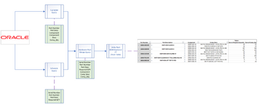
1) The data is coming out of Oracle in 2 different Reports

• Schedule Query (Contains the production Schedule)
• Full BOM Query (Contains the Part Number and Components under the PN as an Exploded BOM - Components inside the PN)

2) Data is queried using Power Query into 2 different dynamic tables per Excel SOP for data queries
3) The Power Queries are Merged into a new query called Hardware Pack Merge Query
4) The Merged query is then used to create a PivotTable called Hrdw Pack BOM Explosion PT (see image)

• Under Values Count of Required Quantity is correct but duplicated
• Sum of Comp_Qty values are correct as is.

The SN is used to verify that no hardware packs / components are duplicated since there can only be a single hardware pack to a specific Part Number.

Here is the general data flow map

 

[mintjulep]

At least one of us doesn't understand your requirements.

That makes it a lot harder to help.