conditional formatting on criteria in multiple columns with nulls

[DSaba10]

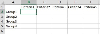
I'm attempting to create some conditional formatting for the example screen below:

What I'd like to see is if I accidentally enter duplicate criteria marks (with any value) in any of the cross cells for a particular "Group" B-F will highlight with a color.

I was able to create something similar for a different range of values, but it required that every cell in a row had a value. Something like:

=COUNTIFS($B$2:$B$5, $B2, $C$2:$C$5, $C2, $D$2:$D$5, $D2, $E$2:$E$5, $E2, $F$2:$F$5, $F5)>1

Again, the above will work if every cell in each of those rows has a value, but if row 2 has C2 with an X and row 4 also only has C4 with an X, I'd like those two rows to be highlighted... of course while ignoring the null values.

Thanks for any thoughts or help.

 

[SkipVought]

Hi,

Simplest way in column G make a helper column with formula
[tt]
G2: =COUNTA(B2:F2)
[/tt]
If the return value is greater than 1, then younhave multiple Xs.


Alternatively, using Conditional Formatting...
[tt]
B2: =COUNTA($B2:$F2)>1
[/tt]
...and Format

Skip,
[sub]
Just traded in my OLD subtlety...
for a NUance![/sub]

 

[DSaba10]

Close, but not quite what I'm looking for. I want to cross reference B2:F2 against every other row. If the entire set of values in row 2 is duplicated again on row 3 (or 4, or 5, etc), I need them both to highlight. Not just one row at a time.

 

[SkipVought]

Are stating that the equation for conditional formatting is ONLY that no Criteria (in your columns) can be duplicated. So that no two gropus can have the same single criteria?

Skip,
[sub]
Just traded in my OLD subtlety...
for a NUance![/sub]

 

[DSaba10]

That's correct. No two groups should have the same criteria.

 

[SkipVought]

[tt]
B2: =COUNTA(B$2:B$5)>1
[/tt]

Skip,
[sub]
Just traded in my OLD subtlety...
for a NUance![/sub]

 

[DSaba10]

This looks like your previous example except instead of duplicates in a row it's now duplicates in a column. I want both row and column. It needs to take B, C, D, E and F all into consideration at the same time and validate it against all subsequent rows of B:F

EX:

Group 1 has B, D, F checked.
Group 2 has B, C, E, F checked.
Group 3 has B, D, F checked.

I'd like group 1 and 3 to be highlighted as it is showing duplicate criteria.

 

[SkipVought]

Thats why I specifically stipulated “ONLY” in my clarification!

How about a Programmer take a shot at putting those two solutions together?

The report back what worked or not.

Skip,
[sub]
Just traded in my OLD subtlety...
for a NUance![/sub]

 

[DSaba10]

I'm not sure if that's some kind of swipe at me, but I'm thinking it is and not really appreciated. I understand your examples and the use of COUNTA() functioning. Per my OP I've tried using COUNTIFS as I'd like the values to be compared not just whether or not it has a value or not, but if the values match. So I know I need to use some variation of COUNTIF/COUNTIFS to track this information but I've not yet been able to get this to function without every cell having a value. All I need to know is how in COUNTIF(range, criteria), to have it consider a cell even if it is blank, but not if the entire row is blank. Maybe I chose my words poorly in my original post. I don't appreciate being made to feel dumb though. Also, I may have the tag of "Programmer" on here, but I'm by no means any kind of expert with Excel, hence why I came here.

 

[SkipVought]

B2: =OR(COUNTA($B2:$F2)>1,COUNTA(B$2:B$5)>1)

Skip,
[sub]
Just traded in my OLD subtlety...
for a NUance![/sub]

 

[DSaba10]

My solution was a two parter:

Conditional Format 1:

=COUNTBLANK($B2:$F2)=5

Each cell has 5 options for criteria, so if all 5 are blank this will make sure the row has no fill color.

Conditional Format 2:

=COUNTIFS($B$2:$B$5, IF(ISBLANK($B2),"", $B2), $C$2:$C$5, IF(ISBLANK($C2), "", $C2), $D$2:$D$5, IF(ISBLANK($D2), "", $D2), $E$2:$E$5, IF(ISBLANK($E2), "", $E2), $F$2:$F$5, IF(ISBLANK($F2), "", $F2))>1

This will turn the duplicate rows red based on value.