Calculate amt due 1

[OCM]

Greetings,

Given my sample workbook in Sheet1, I would like to calculate the amount due by subtracting the total collection amt from one of the settlement #1 per CustID. If the settlement #1 is blank, (e.g., customer #6 – Customer #8, then use settlement #2 to perform the calculation.

Amount due = Settlement #1 - sum of collection amt. If the amount is not entered in settlement #1, then use settlement #2 – sum of collection amt. If the amount is $0.00, then display “no amount due”



On sheet2, I’d like to show the result (attached).



Any feedback?



TIA

 

[gbaughma]

Yeah... my feedback would be "We don't do homework."

 

[combo]

With a layout as in the workbook, IMHO the only way is to manually arrange output.

If it is possible to rearrange data, I would use:

column	example/remarks
CustID	C004200
Name	Cusomer #4
SettlementID	#1, #2, ...
Type	Settlement, collection
Amount	use negative in one of types (for proper sums)
Date	add start date for Settlement

After this a simple pivot table can aggregate required values up-to-date.
More flexible analysis could combine customer+settlement data in one table and related collection in the second one. In this case pivot table could return report from tables connected in Power Query.

 

[SkipVought]

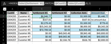
Here's a solution using Structured Tables. First convert your table on Sheet 1 to a structured table via Insert > Tables > Table...

Here are the formulas
Settlement #1: =INDEX(Table1[Settlement '#1],MATCH([@CustID],Table1[CustID],0),1)
Settlement #2: =INDEX(Table1[Settlement '#2],MATCH([@CustID],Table1[CustID],0),1)
Collection Amt.: =SUMPRODUCT((Table1[CustID]=[@CustID])*(Table1[Collection Amt.]))
Amount Due: =IF(([@[Settlement '#1]]+[@[Settlement '#2]])-[@[Collection Amt.]]=0,"no amount due",([@[Settlement '#1]]+[@[Settlement '#2]])-[@[Collection Amt.]])
Here' your workbook modified...

 

[OCM]

Hi Skip,

Thank you.
Here' your workbook modified... do you mean to attach a modified workbook, or are you referring to the screenshot you provided.

TIA,

 

[OCM]

Hi Skip,
I would like to alter my original post a bit and include the itemized collection amounts and display the amount due per CustID at the bottom. In the attached sample, I created 'Amount due' column and manually calculated the collection amounts and the amount due to show the expected result.


TIA

Regards,