User Error Logs / Matrix / Array / ? - VBA Excel

[remeng]

Hi All;

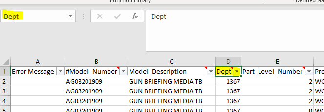
I don't know where to start on this project and was hoping for some guidance. I've included a photo to help explain what I am trying to do.

I have a list of information on a "data" sheet. The headers are also listed on an "error rules" sheet (see picture). I have some engineers that need to be able to check their data based on conditions specified on the "error rules" sheet. Each rule has its own row. The reason for the "error rules" sheet is so that the engineers can add rules as production needs change. Currently they are using very complex macros that are difficult to edit (prior to my time). We are talking about 20+ nested IF statements in the formula bar. Messy to say the least.

What I would like to do is have the engineer be able to add rules to the "error rules" sheet as either an OR statement or an AND statement.

The engineer would select AND or OR, the macro looks at all the cells in the row and evaluates each one against the data row in the "data" sheet. The headers in each sheet must match since I am concerned that someone will add columns to the "error rules" sheet that aren't matched to the "data" sheet table layout exactly. I'd like this to be as robust as reasonably possible.

I am going to have them use 1 line per rule. Most of the statements are going to be AND statements. Only a few will be OR statements. The engineer will not be able to use an AND an OR statement in the same row to elevate confusion.

I will have a LOOP so that each row on the "data" sheet will be checked against all of the rules on the "error rules" sheet.

Example 1:​

DEPT = 100 AND Part_Description = Fred​

The macro goes to the first row and checks to see if Dept = 100 and Part_Description = Fred​

IF conditions = TRUE then insert Error Message "Test 1 - Both Met" into a specified location​

Example 2:​

#Model_Number = ABC​

Part_Level_Number = 2​

The macro goes to the first row and checks to see if #Model_Number = ABC or Part_Level_Number=2​

IF conditions = TRUE then insert Error Message "Test 2 - 1 or Both Met"​

Example 3:​

Error Code 1 and 2 are met. Both Error Message need to be entered into a specified cell. There might be 10+ errors that need to be added to the same cell​

Thought process:

1) Count rows in "data" sheet to determine how many loops to be performed on rule checking and set
2) Count rows in "error rules" sheet to determine the total number of rules that need to be checked
3) Start with Row 1 of "data"
4) check the "data" row for the AND / OR rules line by line on the "error rules" sheet
5) return all record errors to a cell / note on the "data" sheet
6) LOOP process to all records have been validated

What is the best way to start? Matrix, Array, something else? I KNOW that this is going to be the most complex VBA project I have ever undertaken.

Thanks,

Mike

 

[remeng]

Update:

After talking with the engineers, they'd like to have formulas per rule line instead so that they can have more complex rules. This actually will be easier I think for the programing too.

If I set the column header cells range name to equal the column header and use those in the formulas, will that resolve the issue if someone changes the sequencing of the columns too?

is this now a simple loop statement were I loop the cell formula and do a return of the error and highlight the effected cells?

Thanks,

Mike

 

[SkipVought]

Mike,

Keep your heading values consistent. The order should be irrelevant.

This is not a particularly complex project. One step at a time.

AND--Are usually all in one row. If any test value fails, the AND is FALSE.
OR--Are usually in a separate row.



Skip,
[sub]
Just traded in my OLD subtlety...
for a NUance![/sub]
"The most incomprehensible thing about the universe is that it is comprehensible" A. Einstein

 

[remeng]

Hi,

So it seems like I will need to use the FIND function in the data tab to locate the specific column for the IF / THEN statement to run on. I don't have a problem with that. What I'd like to understand is, if I have a custom formula on the error rules sheet, what is the best way to apply it so that the formula loops on the column?

I'm stuck on how to take a formula that isn't defined by any range in one sheet and program it to assign itself to the column in another sheet.

So I guess it is something like if a formula is based on the "data" sheet column headers, it will check the associated columns based on their headers and perform a loop check for all the rows.

Example:

Column A = Material
Column B = Color
Column C = Dept

The general formulas are located on the Error Rules sheet

Formula outline​

if Material > 0 then color needs to be > NULL and Dept = 10 else return error in A some row number #​

Is this even possible?

Thanks,

Mike

 

[Andrzejek]

If you are looking for an outcome that looks something like this:

[pre]
A B C D
Material Color Dept Error?
1 Blue 10 OK
2 10 Error
0 Black 9 Error
5 Red 11 Error
[/pre]
"if [blue]Material > 0[/blue] then [green]color needs to be > NULL[/green] and [red]Dept = 10[/red] else return error in A some row number #"
Then, I 'translated' your 'Formula outline' to this (in cell D2 and down):
[tt] =IF(AND(AND([blue]A2>0[/blue], [green]LEN(B2)>0[/green]), [red]C2=10[/red]), "OK", "Error") [/tt]

---- Andy

"Hmm...they have the internet on computers now"--Homer Simpson

 

[remeng]

Hi Andy,

It is sort of what I am looking at. I think it is a little hard to explain. Let me try again though.

Here is the code I started to work on. It pulls the header name from the "definitions" sheet and finds it in the "test_data" sheet.

After the column number is returned, the formula will be able to have a start point. Since the formula doesn't know where in "test_data" it is initially being applied to, how do I set the formula in the "definitions" sheet to handle the columns being variable?

The columns could be like:

Material | Color | Dept

or

Color | Material | Dept

or

Dept | Material | Color

etc.

so in the cell where the rule is kept, it would be something like:

= if( Material > 0 and color > NULL and Dept = 10, , return error in A some row number #)

Sub find_header()

'********  WORK IN PROGRESS *******

'macro finds header from definition and returns the column number / id


condition_terms = 2

records = ActiveWorkbook.Sheets("definitions").Cells(Cells.Rows.Count, "A").End(xlUp).Row

Do While condition_terms <= records

 
    search_term = Sheets("definitions").Cells(condition_terms, 1).Value
    
    
    
    Sheets("test_data").Select
    Cells.Find(What:=search_term, After:=ActiveCell, LookIn:= _
        xlFormulas2, LookAt:=xlWhole, SearchOrder:=xlByRows, SearchDirection:= _
        xlNext, MatchCase:=False, SearchFormat:=False).Activate
        
subject_column = ActiveCell.Column
info = ActiveCell.Value
        
        
condition_terms = condition_terms + 1
        
Loop


End Sub

I hope this helps explain it a little better.

Mike

 

[remeng]

Ok. Well I have made a significant amount of progress on this and have got the values to return correctly based on what the column and row are defined as using NAME for the cell name. I think I only need one item left to be tackled and I don't know how to go about it.

since the formula will be based off of a series of values, is there a way to call a macro from inside a IF formula located in a cell? I also do not want it to be run until a button is pressed. Is this possible and how can it be done without turning off Auto Calculate?

so here is what I have so far:

The cell has a NAME defined

Here is the code to set the NAME for each cell in the table where the data is stored

Sub name_set() 'working NAME set based on cell value

Call DeleteNames

i = 3 ' "definitions" Skip the "Error Message" and "#Model_Number" columns due to "Error Message" not having a definitions and "#Model_Number" being an invalid cell NAME.  Sets values in the "data" sheet
d = 3 ' starting location for the definitions.  Starts after "#Model_Number" row due to "#Model_Number" being an invalid cell NAME

total_def = ActiveWorkbook.Sheets("definitions").Cells(Cells.Rows.Count, "A").End(xlUp).Row 'counts the number of column definitions on the "definitions" sheet


Do While i <= total_def 'sets the loop to cycle through the "definitions" until the number of "definitions" has been reached


    Dim location As Range 'value used to sheet initial cell where the NAME originates from
    
    Set location = ActiveWorkbook.Sheets("data").Cells(1, i) 'Sets the target for the actual cell that you want to be NAMEd


    location.Name = ActiveWorkbook.Sheets("definitions").Cells(d, 1).Value 'Vale where the name will be generated from

i = i + 1
d = d + 1

Loop

End Sub

Here is the code to pull the value from the table based on the column NAME value.

Sub value_return_dept() 'returns the value in the "data" table under a specified column


' "dept" will be called out in a formula within a cell's IF statement

bob = Range("dept").Row 'returns the row address for the "dept" column
sam = Range("dept").Column 'returns the column address for the "dept" column

Do While bob <= 100 ' 100 will be defined by the total number of rows in the data table.  Code will be changed in the future.  100 is a place holder for testing.

fred = Cells(bob + 1, sam).Value ' returns the value inside the cell

bob = bob + 1 ' selects the next row

Loop

End Sub

what I'd like to do is have a cell call the value_return_dept macro and check the conditions in an IF formula defined in a cell where the engineer can enter the NAME and set the conditions for the IF statement / formula. Again, this is to be triggered by a button and not when the cell is exited.

Thanks for the help and support.

Mike

 

[remeng]

Hi,

I've come a long way on this problem. I am now having an error in the current_error_msg adding the new_new_error_msg when the current_error_msg is not blank. My code process the new formula correctly and provides the new error message correctly, but will not add it to the error message column without overwriting the current value. I know the issue is in the IF current_error_msg <> "" of the code. How can I fix it?

Thanks for the help!

Mike

Sub error_check() ' evaluates rules and adds error log to record

'Application.ScreenUpdating = False

ActiveWorkbook.Sheets("data").[data[Error Formula]].Formula = ""
ActiveWorkbook.Sheets("data").[data[Error Message]].Formula = ""


r = 2

total_rules = ActiveWorkbook.Sheets("error rules").Cells(Cells.Rows.Count, "C").End(xlUp).Row 'Column "C" / #Model_Number is selected to count due to Column "Error Messge" and Column "Error Formula" being added

material_value = IsEmpty(ActiveWorkbook.Sheets("data").[data[@[Material]]].Value)

Do While r <= total_rules

    If material_value = False Then
    
    Else
    
        ActiveWorkbook.Sheets("data").[data[Error Formula]].Formula = ActiveWorkbook.Sheets("error rules").Cells(r, "B").Value
        
        current_error_msg = ActiveWorkbook.Sheets("data").[data[@[Error Message]]].Value
    
        new_error_msg = ActiveWorkbook.Sheets("data").[data[Error Formula]].Value
 

 
    
    End If
    
    
    If current_error_msg <> "" Then
        
        
                combined_error_msg = current_error_msg & Chr(10) & new_error_msg
                
                ActiveWorkbook.Sheets("data").[data[Error Message]].Formula = combined_error_msg
            
    Else
            
                ActiveWorkbook.Sheets("data").[data[Error Message]].Formula = new_error_msg
        
        
    End If

ActiveWorkbook.Sheets("data").[data[Error Formula]].Formula = ""

r = r + 1

Loop



'Application.ScreenUpdating = True

End Sub

 

[Andrzejek]

will not add it to the error message column without overwriting the current value

current value = current value & new error message
or in other words:
error message column = error message column & new error message

---- Andy

"Hmm...they have the internet on computers now"--Homer Simpson

 

[remeng]

Hi Andy,

The error formula would be an IF statement that returned an error message in the "Error Formula" column (inside a table called "data") from another sheet called "error rules". This section of the code works.

The code then takes the value from the "Error Formula" cell and pastes it into the "Error Message" cell. This section of the code also works.

Once the script goes from r = 2 to r = 3, the next rule located in the "error rules" sheet is run. This works correctly.

What is broken is that the section of the code where it copies the current error in the "Error Message" cell with the new error message generated in the "Error Formula" cell. It appears that the script isn't able to determine that there is a value already located in the "Error Message" cell which causes it to go to the ELSE statement instead of the combine_error_msg formula.

If current_error_msg <> "" Then
        
        
                combined_error_msg = current_error_msg & Chr(10) & new_error_msg
                
                ActiveWorkbook.Sheets("data").[data[Error Message]].Formula = combined_error_msg
            
    Else
            
                ActiveWorkbook.Sheets("data").[data[Error Message]].Formula = new_error_msg
        
        
    End If

 

[Andrzejek]

If[tt] current_error_msg[/tt] is a String, or something that you could display, I would try:

[red]Debug.Print current_error_msg[/red]
If current_error_msg <> "" Then
    combined_error_msg = current_error_msg & Chr(10) & new_error_msg
    ActiveWorkbook.Sheets("data").[data[Error Message]].Formula = combined_error_msg
Else
    ActiveWorkbook.Sheets("data").[data[Error Message]].Formula = new_error_msg
End If

and stop and SEE what's in there.

---- Andy

"Hmm...they have the internet on computers now"--Homer Simpson

 

[remeng]

Andy,

As I expected based on the results on the second loop current_error_msg = "" even though there are values in the "Error Message" column in the formatted table.

It's weird since the original code works if there is no other code except this:

current_error_msg = ActiveWorkbook.Sheets("data").[data[@[Error Message]]].Value
new_error_msg = ActiveWorkbook.Sheets("data").[data[@[Error Formula]]].Value

combined_error_msg = current_error_msg & Chr(10) & new_error_msg

ActiveWorkbook.Sheets("data").[data[@[Error Message]]].Value = combined_error_msg

The current embedded code returns the proper values, just won't transfer them to the Error Message cell correctly.

 

[Andrzejek]

Looks like you are wiping out [tt]current_error_msg[/tt] somewhere...

Would that help?

If [blue]ActiveWorkbook.Sheets("data").[data[@[Error Message]]].Value[/blue] <> "" Then
    combined_error_msg = current_error_msg & Chr(10) & new_error_msg
    ActiveWorkbook.Sheets("data").[data[Error Message]].Formula = combined_error_msg
Else
    ActiveWorkbook.Sheets("data").[data[Error Message]].Formula = new_error_msg
End If

---- Andy

"Hmm...they have the internet on computers now"--Homer Simpson

 

[remeng]

Hi Andy,

I tried your code and I get the exact same thing. What are the different terms for "" or having no value in the cell? Maybe it is showing as blank but it is something else? Also, could cell format have something to do with it? For instance text versus general format?

Thanks,

Mike

 

[Andrzejek]

Unless you have some unprintable 'stuff' in a cell, like Chr(10), Chr(13), Tab character and such, "" is usually sufficient to check if there is anything in a cell.
You may use [tt]Len(Trim(current_error_msg))[/tt] but my guess is you will have the same outcome.
So it looks to me there isn't anything in the cell or variable, no matter how you check it.

could cell format have something to do with it?

No. Format does not change anything in the cell itself. Format just changes the display of what's in it.

---- Andy

"Hmm...they have the internet on computers now"--Homer Simpson

 

[combo]

If you use "@" in structured table references, also in VBA, you always refer to active cell in active sheet row. Your loop will populate single cell. So you need either to select cell in proper row when you loop, or refer to specific cell of the table (if you need this): [tt]ActiveWorkbook.Sheets("data").ListObjects("data").ListColumns("Error Message").DataBodyRange(i)[/tt].

combo

 

[remeng]

Hi Combo,

I think you might be able to help with this issue since I am researching the @ symbol currently, but don't fully understand the concept. I am currently reading this VBA article [URL unfurl="true"]https://docs.microsoft.com/en-us/office/vba/excel/concepts/cells-and-ranges/range-formula-vs-formula2[/url]

here is my error rules formulas on the "error rules" sheet. Is there an issue between the following rule formula and the vba in the background?

Column B = Formula
Column C = Error Message

B2
=IF(data[@Material]="","",IF(LEFT(TRIM([@Material]),2)<>"00","",'error rules'!C$2))

C2
Bare Core must be 5 x 8 and not 8 x 5

B3
=IF(data[@Material]="","",IF(LEFT(TRIM([@Material]),2)<>"LF","",'error rules'!C$3))

C3
Part number starts with LF

here is my full vba code currently:

Sub error_check() ' evaluates rules and adds error log to record

'Application.ScreenUpdating = False

ActiveWorkbook.Sheets("data").[data[Error Formula]].Formula = ""
ActiveWorkbook.Sheets("data").[data[Error Message]].Formula = ""


r = 2

total_rules = ActiveWorkbook.Sheets("error rules").Cells(Cells.Rows.Count, "C").End(xlUp).Row 'Column "C" / #Model_Number is selected to count due to Column "Error Messge" and Column "Error Formula" being added

material_value = IsEmpty(ActiveWorkbook.Sheets("data").[data[@[Material]]].Value)

Do While r <= total_rules

    If material_value = False Then
    
    Else
    
        ActiveWorkbook.Sheets("data").[data[Error Formula]].Formula = ActiveWorkbook.Sheets("error rules").Cells(r, "B").Value
        
        current_error_msg = ActiveWorkbook.Sheets("data").[data[@[Error Message]]].Value
    
        new_error_msg = ActiveWorkbook.Sheets("data").[data[Error Formula]].Value
 

 
    
    End If
    
Debug.Print current_error_msg
    
    If current_error_msg <> "" Then
        
        
                combined_error_msg = current_error_msg & Chr(10) & new_error_msg
                
                ActiveWorkbook.Sheets("data").[data[Error Message]].Formula = combined_error_msg
            
    Else
            
                ActiveWorkbook.Sheets("data").[data[Error Message]].Formula = new_error_msg
        
        
    End If

ActiveWorkbook.Sheets("data").[data[Error Formula]].Formula = ""

r = r + 1

Loop



'Application.ScreenUpdating = True

End Sub

 

[combo]

For structured tables it means "the same row as for formula cell". Something like relative formulas in R1C1 notatation, or names after removing any of "$" signs in reference - they became relative, keeping the same RC distance.
No problem when you write formula in worksheet and refer to structured table cell in the same row, the address changes to structured table reference and remains the same when you copy up/down, but refers to different row.
In VBA, when you refer to structured table data with "@" in reference, the code assumes that you mean the same row as active cell.

As for your code, still working with structured table, you can get table data size from [tt]ActiveWorkbook.Sheets("data").ListObjects("data").DataBodyRange.Rows.Count[/tt] and loop the rows using [tt]For...Next[/tt] instead [tt]Do...Loop[/tt]. You can also refer to data rows as in the code in my previous post ([tt]DataBodyRange[/tt] is a range, so you can refer to its cells as for other ranges). References with @ are not fixed and depend on active cell.

Also, note that [tt]ActiveWorkbook.Sheets("data").[data[Error Formula]].Formula = ""[/tt] cleans the whole column, [tt]ActiveWorkbook.Sheets("data").[data[@[Error Formula]]].Formula = ""[/tt] only the cell in active cell's row.

combo

 

[remeng]

Hi Combo,

Thank you for the fantastic explanation on how @ works.

I am a little confused as to what you are recommending with regards to For / Next instead of Do / Loop. I think you mean that I should count the number of rows in the "data" table and then run the code as a loop per line. Is that correct? If so, what is the advantage to that over the current code method were it runs the rules throughout the entire table at one time?

The formulas return the correct results per loop, but the problem is that at the start of the next loop, the error message is deleted from the "Error Message" column and when the new error message is generated, the new one is not added to the end of the previous message.

With regards to ActiveWorkbook.Sheets("data").[data[Error Formula]].Formula = "" being used, I am using it to clear the formula prior to the next formula being brought in from the "error rules" sheet.

Also, while I am starting to understand the way this is working in more detail, how do I actually correct it? I am playing in waters well beyond the Mariana Trench in my understanding of VBA.

What am I still doing incrrectly?

Thanks,

Mike

 

[combo]

If you plan to process all data rows, for me it is more readible:

[pre]With ActiveWorkbook.Sheets("data").ListObjects("data")
TotalRows = .DataBodyRange.Rows.Count
For i = 1 To TotalRows
' process error_msg
current_error_msg = .ListColumns("Error Message").DataBodyRange(i)
new_error_msg = .ListColumns("Error Formula").DataBodyRange(i)
' ...
Next i
End With[/pre]

In your code, test in break mode or execute line by line:
[tt]ActiveWorkbook.Sheets("data").[data[Error Formula]].Formula = ""
ActiveWorkbook.Sheets("data").[data[Error Message]].Formula = ""[/tt]
Clears "Error formula" and "Error message" data, it's ok.

[tt]current_error_msg = ActiveWorkbook.Sheets("data").[data[@[Error Message]]].Value[/tt]
Assigns to current_error_msg value from row same as for active cell, depend on user's selection.

[tt]new_error_msg = ActiveWorkbook.Sheets("data").[data[Error Formula]].Value[/tt]
I haven't check this, from first data cell in column?

Etc.

combo