Match Lookup and Copy Column

[Eitel13]

Hi All,

I have 1 main workbook with one sheet only containing user data
This worksheet has 11 columns
The column headings are as follows

Main​

wbk1​

wbk2​

wbk3​

.... etc

I have another workbook with 10 sheets; each sheet also containing user data
Each worksheet has 2 columns - Employee Number & Status ("Active" or "Inactive")
Each worksheet is named as follows

wbk1​

wbk2​

wbk3​

.... etc
I need to do a lookup with the employee number (found in column A starting at cell A3 in the MAIN workbook) and search through the other 10 worksheets for a match.
When a match is found, under the relevant column in the main workbook, the status column should be copied

Example:

Main Workbook has 11 Columns

Column 1 - Employee Number​

Column 2 - wbk1​

Column 3 - wbk2​

We take the Employee Number in Column 1 of our main workbook, open our second workbook, search for the Employee Number in wbk1 and if there is a match, then under Column 2 in the main workbook, we put the text from the status column (which would be either "Active" or "Inactive"). This needs to be repeated for every employee number in the main workbook through every sheet in the second workbook.

If this sounds very confusing, please ask and I will try to make it more simple.

I do not yet have sample code, however I am working on it.

 

[Andrzejek]

It would be nice to have your Excel files as attachments to your post.
As well as another file with the desired outcome.


---- Andy

There is a great need for a sarcasm font.

 

[SkipVought]

Hi,

This is confusing because you made contradictory assertions about the Main workbook:

I have 1 main workbook with one sheet only containing user data
This worksheet has 11 columns
The column headings are as follows
Main
wbk1
wbk2
wbk3
.... etc

...and...

Main Workbook has 11 Columns
Column 1 - Employee Number
Column 2 - wbk1
Column 3 - wbk2

So we’re not certain about exactly what your problem is and how to suggest a solution because you don't seem to know how to explain your problem clearly.

Secondly, the apparent structure of your second workbook, that is each wkn sheet having two columns, Employee Number and Status, and that sheet name corresponding to the column headings in the Main workbook, is a horrible design, because Excel has no native features for searching multiple sheets. Therefore, by creating such a workbook, you have shot yourself in the foot, making the solution extremely difficult for yourself. A much better design for the other nameless workbook would be ONE sheet with these columns:
[tt]
Wk Number, Employee Number, Status.
[/tt]
In fact having this data in another workbook adds a level of unnecessary complexity that would be handled much easier if ALL this data were in the Main workbook, in one sheet.

Waiting on your reply.

Skip,
[sub]
Just traded in my OLD subtlety...
for a NUance![/sub]

 

[SkipVought]

Here's a one workbook solution.

Here's the formula assuming a Structured Table in the Status sheet named tStatus...
[tt]
B2: =IFERROR(INDEX(tStatus[Status],SUMPRODUCT((tStatus[Wk Number]=B$1)*(tStatus[Employee Number]=$A2)*(ROW(tStatus[Status])))-1,1),"")
[/tt]

If the Status table is in another workbook, then the formula would simply reference that workbook in addition to the table/range.


Skip,
[sub]
Just traded in my OLD subtlety...
for a NUance![/sub]

 

[Eitel13]

Hi Skip,

Apologies for the contradictions in my column headings, this was an oversight when typing up my question... The column heading in the main workbook should be Employee Number, wbk1, wbk2 and so on..

Also apologies that many of my posts seem to contain quite a large amount of unnecessary work-arounds to get to my end goal.... At the time of posting the questions, it seems to make sense in my head

I am happy to have only one workbook with all the data in it

Lets see if understand you correctly:

I have one workbook with 2 Sheets: ONE & TWO

In worksheet ONE I have 11 Columns: EmpNumber, wbk1, wbk2, wbk3 and so on

In worksheet TWO I have 3 Columns: wk number, EmpyNum, Status

NOTE: The names wbk1, wbk2 and so on, are not the actual names - I'm simply using those names for the sake of posting the question; So I cannot have a loop that goes through the names - wbk(i)...

Here is the "structure" I have in mind:

Worksheet 1:

Column 1​

Column 2​

Column 3​

Employee Number​

wbk1​

wbk2​

1234​

Active​

Inactive​

5678​

Active​

Active​

2468​

Inactive​

Inactive​

 

[SkipVought]

Did you download my workbook?

Your structure of sheet one is my structure.

Skip,
[sub]
Just traded in my OLD subtlety...
for a NUance![/sub]

 

[SkipVought]

In the attached workbook, I used your Employee Numbers...

Notice that the Employee Number column (field) has a Number Format of TEXT in BOTH tables.

faq68-6659

Skip,
[sub]
Just traded in my OLD subtlety...
for a NUance![/sub]

 

[Eitel13]

Hi Skip,

I coincidentally did not see your attachment before I posted my reply.

Two Questions:

1) How would I get the 10 worksheets into one worksheet with 3 columns? Currently, each worksheet has 2 columns, but how would I get the wk umber in the first column?
2) Can I use the formula you provided and put it into a macro?

The idea here is that there are a few macros, each doing their own part and the user will run a single macro that calls each macro and at the end of it all, the user will have the final sheet in-front of them with EmpNum, wbk1, wbk2 etc..

Thank you for the help!

 

[Eitel13]

Hi Andrzejek,

I apologize, I did not see your post. For whatever reason I cannot upload files to the site. I think there is a block on the network at my workplace that prevents the upload of files to sites.

The idea (in the desired workbook) is that the first column contains the EmpNum, and every column after that contains the workbook name as the header and the status of that EmpNum found in that workbook.

With Skip's idea though, there will only be one workbook with 2 worksheets - worksheet 1 with the above mentioned structure and worksheet 2 with three columns - wk number, EmpNum, Status.

 

[SkipVought]

Currently you have two workbooks. Workbook ONE appears to have a summary of the data in workbook TWO.

Unless there are circumstances of which I an unaware, I’d recommend to simply COPY each sheet of data from workbook TWO and PASTE into the new table in workbook ONE, adding the appropriate wbk number column data for each MANUALLY, since this seems that it is only a ONE TIME operation.

If this is not a ONE TIME operation, but will be ongoing (that is getting NEW DATA from workbook TWO)...

Where does the DATA for workbook TWO come from?

If all the data from workbook TWO were to be transfered to workbook ONE into a three column table, could workbook TWO cease to exist?

Skip,
[sub]
Just traded in my OLD subtlety...
for a NUance![/sub]

 

[Eitel13]

Hi Skip,

Again it has been long since I posted a reply, however, I have some good feedback...

In the other thread I managed to get my workbook 2 created with the multiple sheets inside... The below code combines the multiple sheets into a single summary sheet:

Sub CopySheetNameToColumn()

Dim sh As Worksheet
    Dim DestSh As Worksheet
    Dim Last As Long
    Dim CopyRng As Range

    With Application
        .ScreenUpdating = False
        .EnableEvents = False
    End With

    'Delete the sheet "3rdPartySummary" if it exist
    Application.DisplayAlerts = False
    On Error Resume Next
    ActiveWorkbook.Worksheets("3rdPartySummary").Delete
    On Error GoTo 0
    Application.DisplayAlerts = True

    'Add a worksheet with the name "3rdPartySummary"
    Set DestSh = ActiveWorkbook.Worksheets.Add
    DestSh.Name = "3rdPartySummary"

    'loop through all worksheets and copy the data to the DestSh
    For Each sh In ActiveWorkbook.Worksheets
        If sh.Name <> DestSh.Name Then

            'Find the last row with data on the DestSh
            Last = LastRow(DestSh)

            'Fill in the range that you want to copy
            Set CopyRng = sh.Range("A2", sh.Range("B" & Rows.count).End(xlUp))

            'Test if there enough rows in the DestSh to copy all the data
            If Last + CopyRng.Rows.count > DestSh.Rows.count Then
                MsgBox "There are not enough rows in the Destsh"
                GoTo ExitTheSub
            End If

            'This example copies values/formats, if you only want to copy the
            'values or want to copy everything look at the example below this macro
            CopyRng.Copy
            With DestSh.Cells(Last + 1, "B")
                .PasteSpecial xlPasteValues
                .PasteSpecial xlPasteFormats
                Application.CutCopyMode = False
            End With

            'Optional: This will copy the sheet name in the H column
            DestSh.Cells(Last + 1, "A").Resize(CopyRng.Rows.count).Value = sh.Name

        End If
    Next

ExitTheSub:

    Application.Goto DestSh.Cells(1)

    'AutoFit the column width in the DestSh sheet
    DestSh.Columns.AutoFit

    With Application
        .ScreenUpdating = True
        .EnableEvents = True
    End With

End Sub

Function LastRow(sh As Worksheet)
    On Error Resume Next
    LastRow = sh.Cells.Find(What:="*", _
                            After:=sh.Range("A1"), _
                            Lookat:=xlPart, _
                            LookIn:=xlFormulas, _
                            SearchOrder:=xlByRows, _
                            SearchDirection:=xlPrevious, _
                            MatchCase:=False).Row
    On Error GoTo 0
End Function

Function lastCol(sh As Worksheet)
    On Error Resume Next
    lastCol = sh.Cells.Find(What:="*", _
                            After:=sh.Range("A1"), _
                            Lookat:=xlPart, _
                            LookIn:=xlFormulas, _
                            SearchOrder:=xlByColumns, _
                            SearchDirection:=xlPrevious, _
                            MatchCase:=False).Column
    On Error GoTo 0
End Function

This code produces the layout which we discussed previously..

From here, I copy the worksheet to my main workbook:

Sub CopyThirdPartySheet()

Dim x As Workbook, y As Workbook
Dim ws1 As Worksheet, ws2 As Worksheet

Set x = Workbooks("Terminations Template.xlsx")
Set y = Workbooks.Open("C:\Users\Desktop\3rd Party\Work Folder\New folder\test.xlsx")

Set ws1 = x.Sheets("3rdPartySummary")
Set ws2 = y.Sheets("3rdPartySummary")

ws2.Cells.Copy ws1.Cells
y.Close True


End Sub

Now I am at the part where I need to do the vlookup..

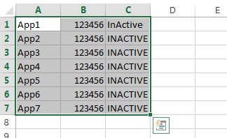
This will be the layout on the 3rdPartySummary sheet:

AppName; EmpID; Status

Then the vlookup needs to match the EmpID from the Consolidated sheet with the EmpID on the 3rdPartySummary sheet.
Copy the AppName (Column A Row 1 on the 3rdPartySummary sheet) and the Status (Column C Row 1 on the 3rdPartySummary sheet), put the AppName into the next available column in Row 1 on the Consolidated sheet and the Status into the corresponding AppName in Row 2

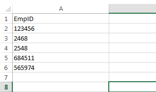
Original Consolidated Sheet:

Original 3rdPartySummary Sheet:

Expected output on Consolidated Sheet:

I have now realized something though...

In the consolidated sheet where the vlookup will be performed, there will sometimes be multiple rows with different empID values..

This could be a possible situation:

In this case, I presume it would be best to do the vlookup for one empID and produce this result:

Then before the next one is done, a blank row is inserted and the next vlookup is done to produce this:

I highlighted the cells to show that it may be possible that not all empID's will match for each app.. So it might be better to have the AppName in each row for every empID there is??

Alternatively, I don't know how we could produce this output:

Hope this makes sense to you as it did to me.. I pasted screenshots as I cannot seem to upload files..

 

[SkipVought]

Here we are 12 days later. I’ve slept since then and forgotten more than I can remember.

Looking back, I sent you a workbook with a sample STATUS sheet, containing what you refer to as 3rdPartySummary sheet:, WITHOUT THE HEADINGS, AppName; EmpID; Status.

So why did you not include the headings, an integral part of any table? THIS IS A MUST!!!

Going back further, I supplied a formula, referencing the above mentioned table as a Structured Table named, tStatus...
[tt]
B2: =IFERROR(INDEX(tStatus[Status],SUMPRODUCT((tStatus[Wk Number]=B$1)*(tStatus[Employee Number]=$A2)*(ROW(tStatus[Status])))-1,1),"")
[/tt]
Well, all you need do is
1) adding your headings and
2) converting your table to a Structured Table and
3) changing the table name to tStatus (a ONE TIME event),
is to change
Wk Number to AppName and
Employee Number to EmpID.



Skip,
[sub]
Just traded in my OLD subtlety...
for a NUance![/sub]

 

[Eitel13]

Hi Skip,

Thank you again for your help.

Apologies for the confusion with the headings, all the headings are still the same except for Wk Number which has changed to App Name. I had created a new sample workbook in which I changed Employee Number to EmpID - which in actual fact is not correct, the correct one is Employee Number.

I converted the data into a structured table and left it named as Table1 for the sake of testing, so this is what the formula looks like:

=IFERROR(INDEX(Table1[Status],SUMPRODUCT((Table1[App Name]=B$1)*(Table1[Employee Number]=$A2)*(ROW(Table1[Status])))-1,1),"")

It works GREAT!

I genuinely appreciate the effort and all your help Skip, THANK YOU VERY MUCH

I am going to now work on getting the formula used in a macro. If I don't come right, I will post again. Thank you again Skip.