Tek-Tips is the largest IT community on the Internet today!

Members share and learn making Tek-Tips Forums the best source of peer-reviewed technical information on the Internet!

  • Congratulations SkipVought on being selected by the Tek-Tips community for having the most helpful posts in the forums last week. Way to Go!

Hello I need your help can you gi

Status
Not open for further replies.

hasnaoui

Programmer
Oct 25, 2020
11
0
0
TN
Hello
I need your help
can you give me an example in which we solve a stiff problems
with a sparce jacobian

best wiches
 
Hello Hasnaoui,

In my opinion instead of sparse Jacobian you probably mean banded Jacobian.

My question:
Wouldn't it be better for you instead of the old good Fortran, rather to try a more modern solving system like Matlab, Octave, Scilab or Julia - at least at the beginning ?

- Matlab is payed and not cheap, but look how nice you can solve stiff ODEs in it and visualize the solution:

- Octave is similar to Matlab, but free, maybe it doesn't have so much methods for ODEs like Matlab, but it has the LSODE method which is similar to the DVODE using backward differentiation formula (BDF). You can visualize your solution like in Matlab:

- Scilab is similar to Matlab too and free like Octave. It seems that it has the same solver like Octave:

- Julia is a new free language and system for solving mathematical problems. It has solvers for stiff ODEs too, and you can immediately visualize your results like in other systems mentioned above:

I would choose the following route: First, learn how to solve the stiff equations in one or two of the systems described above. Verify if the obtained results meet your expectations and then if you are sure how to do it, maybe you can rewrite the solution in Fortran.


But if you are based on the Fortran-only usage, I would suggest you to look at the following book:
Hairer and Wanner: Solving Ordinary Differential Equations. Stiff and Differential-Algebraic Problems.
It looks like this: You may be able to pick the book from a local library.
And here are some fortran codes for the book available:

I know that book, i have read some parts of it, because during my study i implemented some of the implicit Runge-Kutta stiff solvers described in it in the Pascal programming language. And I used the fortran codes from the book to verify whether my pascal implementation delivers right results...but that was almost 30 years ago :)
 
Hi hasnaoui,

I tried to solve your ODE system in Octave with LSODE method, using the right hand side function and initial conditions you provided in the fortran program here:
Default options of LSODE were used:
Code:
>> lsode_options()

Options for LSODE include:

  keyword                                             value
  -------                                             -----
  absolute tolerance                                  1.49012e-08
  relative tolerance                                  1.49012e-08
  integration method                                  stiff
  initial step size                                   -1
  maximum order                                       -1
  maximum step size                                   -1
  minimum step size                                   0
  step limit                                          100000

Here are the 11 resulting functions y(1), .., y(11) visualised:

hasnaoui_1_6_t2syng.png

hasnaoui_7_11_w0exog.png


Here is the octave script file I used, you can try it:
hasnaoui.m
Code:
printf("System of Stiff Ordinary Differential Equations\n");
printf("by hasnaoui\n");

function YDOT = F(Y, T)
  EXI=0.10;
  C0=EXI-5.0/2.0;
  C1=EXI/2.0-1.0/4.0;
  C2=-0.50;
  C3=-0.50;
  C4=EXI-3.0/2.0;

  GAM=5.0/3.00;
  BETA=EXI/2.0+3.0/4.0;
  GU=5.7D-3;
  EP=0.10;
  ALM=1.0;
  XM=1.00;
  PM=1.0;
  PP=PM*EP+3*XM/ALM**2;
  SM=ALM*PP*GU**0.5;
  RM=PP/EP;
  DEL0=(1-EP**2*(SM**2/2.0+2*(2-BETA)+GU*RM))**0.5;
  QQ=ALM*DEL0*(PP-PM*EP)/2.0/GU**0.5;
  TAU=PP/PM/EP-1.0;
  %VARIABLE DI'INTEGRATION
  YDOT(1) = 1.0;
  %RESISTIVITE MAGNETIQUE
  YDOT(10) = -2.0*Y(1)*exp(-Y(1)**2);
  %
  %VITESSE TOROIDALE
  YDOT(2)=(Y(4)*Y(3)*Y(2)+  ...
      TAU/(1.0+TAU)*(Y(9)*Y(6)/Y(10)-C1/BETA*Y(7)*Y(8))  ...
      -1.0/(1.0+TAU)*Y(3)*Y(10))  ...
      /(2.0*Y(3)*(Y(1)*Y(4)+Y(5)));
  %DENSITE VOLUMIQUE
  YDOT(3)=((EXI-1.0)*Y(3)*Y(4)*EP**2*SM**2*Y(3)*(Y(1)*Y(4)+Y(5))  ...
      -Y(1)*Y(3)* ...
      (C2*SM**2*EP**2*Y(3)*Y(4)**2-Y(3)*DEL0**2*Y(2)**2  ...
      +Y(3)/(1.0+EP**2*Y(1)**2)**1.50+EP**2*C0*Y(11)  ...
      +GU*QQ**2*EP**2*Y(7)*(C1*Y(7)-Y(1)*Y(6)/Y(10))    ...
      +GU/BETA*(Y(9)-Y(1)/BETA*Y(8))*   ...
      (-RM*EP**2/Y(10))*(BETA*Y(4)*Y(9)-Y(8)*(Y(1)*Y(4)+Y(5))))  ...
      -Y(3)*  ...
      (C3*SM**2*EP**2*Y(3)*Y(4)*Y(5)-Y(1)*Y(3)/  ...
      (1.0+EP**2*Y(1)**2)**1.50  ...
      -GU*QQ**2*Y(7)*Y(6)/Y(10)-GU/BETA**2/EP**2*Y(8)*  ...
      (-RM*EP**2/Y(10))*(BETA*Y(4)*Y(9)-Y(8)*(Y(1)*Y(4)+Y(5))))  ...
      -1.0/BETA*Y(3)*Y(9)**(-1.0-1.0/BETA)*Y(8)*  ...
      Y(3)*(1.0+Y(1)**2*EP**2)) ...
      /(Y(3)*(SM**2*EP**2*(Y(1)*Y(4)+Y(5))**2-Y(9)**(-1.0/BETA)*  ...
      (1.0+EP**2*Y(1)**2)));

  %PRESSION
  YDOT(11)=-1.0/BETA*Y(3)*Y(9)**(-1.0-1.0/BETA)*Y(8)+  ...
      Y(9)**(-1.0/BETA)*YDOT(3);

  %EQUILIBRE RADIALE
  YDOT(4)=(C2*SM**2*EP**2*Y(3)*Y(4)**2  ...
      -Y(3)*DEL0**2*Y(2)**2     ...
      +Y(3)/(1.0+(EP*Y(1))**2)**1.50  ...
      +EP**2*C0*Y(11)   ...
      +GU*QQ**2*EP**2*Y(7)*(C1*Y(7)-Y(1)*Y(6)/Y(10))  ...
      +GU/BETA*(Y(9)-Y(1)*Y(8)/BETA)*  ...
      (-RM*EP**2/Y(10))*(BETA*Y(4)*Y(9)-Y(8)*(Y(1)*Y(4)+Y(5)))  ...
      -EP**2*Y(1)*YDOT(11))  ...
      /(EP**2*SM**2*Y(3)*(Y(1)*Y(4)+Y(5)));
  %EQUILIBRE VERTICALE
  YDOT(5)=(C3*EP**2*SM**2*Y(3)*Y(4)*Y(5)-  ...
      Y(1)*Y(3)/(1.0+(EP*Y(1))**2)**1.50  ...
      -GU*QQ**2*Y(7)*Y(6)/Y(10)-  ...
      GU*Y(8)/BETA**2/EP**2*  ...
      (-RM*EP**2/Y(10))*(BETA*Y(4)*Y(9)-Y(8)*(Y(1)*Y(4)+Y(5)))  ...
      -YDOT(11))  ...
      /(EP**2*SM**2*Y(3)*(Y(1)*Y(4)+Y(5)));


  %INDUCTION MAGNETIQUE
  YDOT(6)= (EP**2*Y(1)*((C1-1.0)*Y(6)+C1*Y(7)*YDOT(10))  ...
      -EP**2*(C1*Y(7)*Y(10)-Y(1)*Y(6))*(C1-1.50) ...
      -XM*RM*DEL0/QQ/SM*(1.50/BETA*Y(8)*Y(2)+Y(9)*YDOT(2))  ...
      +XM*RM*EP**2*BETA*Y(7)*Y(4)  ...
      +XM*RM*EP**2*(Y(5)+Y(1)*Y(4))*  ...
      (Y(6)/Y(10)-Y(7)*YDOT(3)/Y(3)))  ...
      /(1.0+EP**2*Y(1)**2);

  YDOT(7)=Y(6)/Y(10);


  %FLUX MAGNETIQUE
  YDOT(8)=(EP**2*(BETA*(2.0-BETA)*Y(9)+(2*BETA-3.0)*Y(1)*Y(8))  ...
      -RM*EP**2/Y(10)*(BETA*Y(4)*Y(9)-Y(8)*(Y(1)*Y(4)+Y(5))))  ...
      /(1.0+(EP*Y(1))**2);

  YDOT(9)=Y(8);

endfunction

Y0(1) = 0.0001;
Y0(2) = 1.0;
Y0(3) = 1.0;
Y0(4) = 1.0;
Y0(5) = 0.0;
Y0(6) = -1.;
Y0(7) = 0.0;
Y0(8) = 0.0;
Y0(9) = 1.0;
Y0(10) = 1.0;
Y0(11) = 1.0;

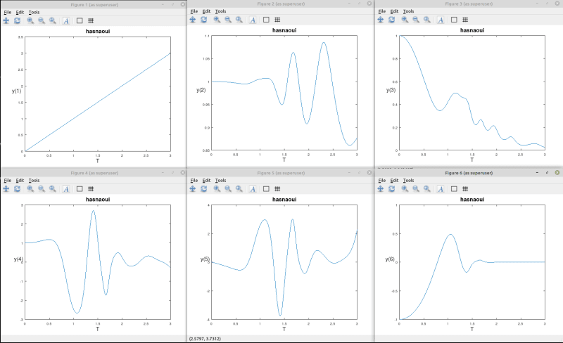
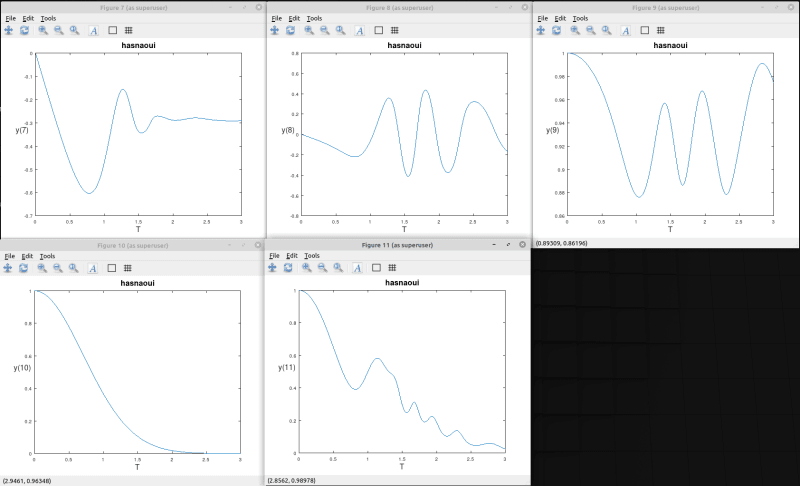
T = linspace(0, 3, 300);

Y = lsode ("F", Y0, T);

for i = 1: columns(Y)
  figure(i);
  plot(T, Y(:,i));
  tit=title ("hasnaoui", "fontsize", 16);
  l=xlabel("T", "fontsize", 16);
  ylabel(sprintf("y(%d)", i), "fontsize", 16, "rotation", 0);
endfor
 
Dear Programmer

Thank you very much for your help

The same results attached to your response are obtained using the dvode code.
My objective is to integrate the stiff equations for large time (infinity).
I don't know if the Lsode allows to resolve the stiff equations for large time

Again, i would thank you for your attention
best regards
 
To see how the method works, i first integrated Van der Pol equation on a very long interval [0, 3000]. That was without problem and I got results like here Then I tried your system but it computed without end.
However, Van der Pol consists only of 2 ODEs and your system of 11 ODEs.
Then, to get some result only for a demo purpose, I integrated it only on the small interval [0, 3].
The integration on longer interval was too slow on my PC. The stiffness of your system probably increases rapidly over longer intervals, the method must then choose very small steps and so the calculation is very CPU intensive.
 
Status
Not open for further replies.

Part and Inventory Search

Sponsor

Back
Top