Compare 2 columns in seperate sheets but same worknook Excel 2016 2

[Cpreston]

Hi

I want to compare 2 columns in a spreadsheet so it highlights any difference by a code

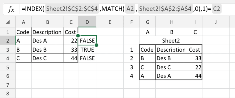
Sheet 1 and Sheet 2 have the same columns

Code Description Cost

By matching the codes in both sheets I want it to highlight in red any cost difference in Sheet 1 compared to sheet 2 where codes are equal.

I then want to able to highlight in an another colour and codes in sheet 1 that do not match in sheet 2

I would like to do this using code. I have tried Conditional Formatting but can seem to get that working. Any ideas at all please.

 

[SkipVought]

Hi,

 I have tried Conditional Formatting but can seem to get that working. Any ideas at all please.

CF works! Chances are, if you did not use a lookup function, your CF failed. What formula did you use?

Skip,
[sub]
Just traded in my OLD subtlety...
for a NUance![/sub]
"The most incomprehensible thing about the universe is that it is comprehensible" A. Einstein

 

[SkipVought]

Here's an example of the formula you might use for a CF...

Notice that Code B is the only one that matches (TRUE) sheet2.

Actually thus is a better formula...
[tt]
D2: =INDEX(Sheet2!C:C,MATCH(A2,Sheet2!A:A,0),1)=C2

[/tt]

Skip,
[sub]
Just traded in my OLD subtlety...
for a NUance![/sub]
"The most incomprehensible thing about the universe is that it is comprehensible" A. Einstein

 

[Cpreston]

Sorry lost me on this one and cannot apply it to my requirements.

I have a sheet called Product Margin where all the codes are listed in column A
The other sheet is called Main Data which again as all product codes in column A

I want to highlight any codes that do not exists between the 2 in red in the sheet Main Data.

Thanks

 

[Andrzejek]

Some sample data representing your issue in the attached Excel file would be nice to have here.
Along with - how the solution would look like.


---- Andy

There is a great need for a sarcasm font.

 

[strongm]

Er ...

By matching the codes in both sheets I want it to highlight in red any cost difference in Sheet 1 compared to sheet 2 where codes are equal.

I then want to able to highlight in an another colour and codes in sheet 1 that do not match in sheet 2

and

I want to highlight any codes that do not exists between the 2 in red in the sheet Main Data.

are inconsistent with each other. Can you please clarify:

1) what colours you want for what
2) on which of the sheets the colours should be

 

[Cpreston]

Hi

I have created a small spreadsheet just to try and get the formula correct

Sheet one in column A as 3 entrys

A1 = Dave
A2 = Mick
A3 = Ian

Sheet 2 in column A as

A1 = Dave
A2 = Mick
A3 = Ian
A4 = Chris

I want to compare both columns and in this case highlight sheet 2 A4 as this name is not in sheet 1

I have managed to get this formula to work in sheet 2 (using your first post)

=INDEX(Sheet2!A1:A4,MATCH(A1,Sheet1!A1:A4,0),1)=A1

However, Sheet 2 A1 to A3 return True, then A4 returns #N/A. Not sure why it comes back with N/A I was expecting false.

The I was going to apply the formula to a CF and try and show sheet 2 A4 in red.. Then try it on my main sheet I am working on. So any ideas why I get #N/A, Thanks

 

[Cpreston]

1) what colours you want for what
2) on which of the sheets the colours should be

I would prefer red and sheet 2. Thanks

 

[strongm]

=INDEX(Sheet2!$A$1:$A$4,MATCH($A1,Sheet1!$A$1:$A$4,0),1)=A1

(and Skip'll be along in a moment to tell us that using structured tables makes this easier … 0-; )

 

[Cpreston]

Strongm thanks for the formula

Using it as below I am still getting TRUE for the 4 that match and #N/A for the one that does not match. Should it be like this or should it be false?

=INDEX(Sheet2!$A$1:$A$4,MATCH($A1,Sheet1!$A$1:$A$4,0),1)=A1

 

[strongm]

This is where the clarity of your requirements becomes key. Skip's formula is designed to flag if there is a price discrepancy between sheet one and sheet two for those items that match codes between sheet 1 and sheet 2. But you are trying to use it to simply match the product codes, which means you don't need INDEX - but you do need to beable to handle the situation when there is no matching code. So something like

=NOT(IFNA(MATCH($A1,Sheet1!$A$1:$A$4,0),FALSE))

Our confusion is understandable because you still have not properly clarified your requirements!

You would prefer RED for WHAT? For mismatched product codes, or for mismatched prices? Or can we forget the prices thing completely?

 

[Cpreston]

Also stronm By the way I am putting the formula in the B column of sheet 2

I put the formula into a conditional format and set it to use red. It highlighted the matching codes but left the one not matching with no fill. I want it to only fill the in-matching ones.
How do I reverse this. Thanks

 

[Cpreston]

Hi

I have attached spreadsheet I want to work called Costs Margin v2.
I have also attached the testing one with names in for you to see

In the Costs Margin v2 I want to highlight in the Refresh Data tab all codes in column A that do not match in Trex Margin column A codes.

Thanks for assistance.

 

[strongm]

Your attached example is still using Skip's formula, which, as stated in my post of 14:59 is does not meet your current requirements (it met some earlier ones, but you seem to have moved off those now). .. Here's your sheet back with my formula from that same post (both in column b and in conditional formatting)

(I should also n ote that there is some synergy between this thread and thread707-1798587)

 

[Cpreston]

Hi

yes sorry about all the messages and nothing very clear, I was trying very hard here to get it working and knew I was close but yet so far away.

Thanks for your code example, I see what it is doing.

 

[Cpreston]

I presume that this cannot be used on the cost margin sheet though.

I have tried it and it does not work.

 

[strongm]

> the cost margin sheet though.

Is this the same as Product MArgin sheet? You've not previously mentioned a cost margin sheet.

In terms of Sheet 1 and Sheet 2, which sheet is this? And do you suddenly need the same behaviour on the 'cost margin' sheet? i.e. highlight names that don't match the other sheet? In which case, sure, it'll work, with a very minor alteration

=NOT(IFNA(MATCH($A1,Sheet1!$A$1:$A$4,0),FALSE))

just change the highlighted sheet name to the name you want

 

[Cpreston]

Sorry in the cost margin sheet

Sheet1 is renamed to Trex Marginb
Sheet2 is renamed to Refresh Data

I change you code as below and have netered it in D2 in the Refresh Data sheet. For some reason when I press enter it opens up a window to select a file from somewhere, if I click the cross to close it it does it again, click the cross and then it populates the D column with #NAME?

=NOT(IFNA(MATCH($A2,Trex Margin!$A$1:$A$1000,0),FALSE))

 

[SkipVought]

=NOT(IFNA(MATCH($A2,Trex Margin!$A$1:$A$1000,0),FALSE))

Regarding your formula,
EDIT the formula.
SELECT Trex Margin!$A$1:$A$1000 in the formula.
The SELECT that range on that sheet.

You will notice the QUOTES around the sheet name because you have a SPACE in your sheet name.

Skip,
[sub]
Just traded in my OLD subtlety...
for a NUance![/sub]
"The most incomprehensible thing about the universe is that it is comprehensible" A. Einstein

 

[strongm]

Caused by the fact that you have a space in the name - so you need to protect it, as it is not unsurprisingly confusing Excel's expression evaluator

=NOT(IFNA(MATCH($A1,'Trex Margin'!$A$1:$A$5,0),FALSE))